SiT: Exploring Flow and Diffusion-based Generative Models with Scalable Interpolant Transformers

We present Scalable interpolant Transformers (SiT), a family of generative models built on the backbone of Diffusion Transformers (DiT)
By carefully introducing the above ingredients, SiT surpasses DiT uniformly across model sizes on the conditional ImageNet 256x256 benchmark using the exact same backbone, number of parameters, and GFLOPs. By exploring various diffusion coefficients, which can be tuned separately from learning, SiT achieves an FID-50K score of 2.06.
In recent years a family of flexible generative model
based on transforming pure noise \(\varepsilon \sim \mathcal{N}(0, \mathbf{I})\) into data \(x_* \sim p(x)\) has emerged.
This transformation can be described by a simple time-dependent process $$
x_t = \alpha_t x_* + \sigma_t \varepsilon
$$
with t defined on \([0, T]\), \(\alpha_t, \sigma_t\) being time-dependent functions and chosen such that \(x_0 \sim p(x)\), \(x_T \sim \mathcal{N}(0, \mathbf{I})\).
At each \(t\), \(x_t\) has a conditional density \(p_t(x | x_*) = \mathcal{N}(\alpha_t x_*, \sigma_t^2\mathbf{I})\),
and our goal is to estimate the marginal density \(p_t(x) = \int p_t(x | x_*) p(x) \mathrm{d}x \).
In most cases, the marginal density \(p_t(x)\) is intractable.
Some previous methods
Diffusion-Based Models.
Diffusion-Based Models
In practice, the model samples the process by learning the gradient of the likelihood \(\nabla \log p_t(x)\) (score) with a generative model \(s_\theta(x_t, t)\) under the score matching objective $$
\mathcal{L}_s(\theta) = \int \mathbb{E}[\Vert \sigma_t s_\theta(x_t, t) + \varepsilon \Vert^2] \mathrm{d}t
$$
Inference is done by solving either a probability flow ODE $$\mathrm{d}X_t = [f(X_t, t) - \frac{1}{2} g^2(t) \nabla \log p_t(x)] \mathrm{d}t $$
or a reverse-time SDE $$
\mathrm{d}X_t = [f(X_t, t) - g^2(t) \nabla \log p_t(x)] \mathrm{d}t + g(t) \mathrm{d} \bar{W}_t
$$
where \(\bar{W}_t\) is a standard Brownian motion with reversed time. Integrating both equations from \(t = T\) to \(t=0\) with initial condition of a Gaussian noise will push to a data sample approximating \(p(x)\).
Stochastic Interpolant and Flow-Based Models.
Stochastic Interpolant and other Flow-Based models
Furthermore, these models use a simpler probability flow ODE for inference
\[\begin{align*}
\mathrm{d}X_t &= \underbrace{[f(X_t, t) - \frac{1}{2} g^2(t) \nabla \log p_t(x)]}_{\text{directly learn this}} \mathrm{d}t \\
\implies \mathrm{d}X_t &= v(X_t, t) \mathrm{d}t
\end{align*}\]
where the velocity \(v(X_t, t)\) is estimated by the flow matching objective $$
\mathcal{L}_v(\theta) = \int \mathbb{E}[\Vert v(X_t, t) - \dot \alpha_t x_* - \dot \sigma_t \varepsilon \Vert^2] \mathrm{d}t
$$
Intuitively, this can be viewed as predicting the velocity of a particle starting moving from some \(\varepsilon\) at time \(t\).
We summarize the components of the above models in the following table:
| Diffusion-Based | Flow-Based | |
|---|---|---|
| \( t \) | \(\{0, \cdots, T\}\) (DDPM |
\([0,1]\) |
| \( \mathcal{L}(\theta) \) | \( \mathcal{L}_s \sim \Vert \sigma_t s_\theta(x_t, t) + \varepsilon\Vert^2 \) | \( \mathcal{L}_v \sim \Vert v_\theta(x_t, t) - \dot \alpha_t x_* - \dot \sigma_t \varepsilon \Vert^2 \) |
| \( x_t \) | \( \alpha_t x + \sigma_t \varepsilon \) | \( \alpha_t x + \sigma_t \varepsilon \) |
| ODE | \( \mathrm{d}X_t = [f(X_t, t) - \frac{1}{2} g^2(t) \nabla \log p_t(x)] \mathrm{d}t \) | \( dX_t = v(X_t, t) \) |
| SDE | \( dX_t =[f(X_t, t) - g^2(t) \nabla \log p_t(x)] \mathrm{d}t + g(t) \mathrm{d} \bar{W}_t \) | ? |
From the above table, we summarize the design space into four components.
| Model | Params(M) | Training Steps | FID \(\downarrow\) |
|---|---|---|---|
| DiT-S | 33 | 400K | 68.4 |
| SiT-S | 33 | 400K | 57.6 |
| DiT-B | 130 | 400K | 43.5 |
| SiT-B | 130 | 400K | 33.5 |
| DiT-L | 458 | 400K | 19.5 |
| SiT-L | 458 | 400K | 17.2 |
| DiT-XL | 675 | 400K | 9.6 |
| SiT-XL | 675 | 400K | 8.6 |
| DiT-XL(cfg=1.5) | 675 | 7M | 2.27 |
| SiT-XL(cfg=1.5) | 675 | 7M | 2.06 |
To investigate such performance improvement, we gradually transition from a DiT model, a typical denoising diffusion model (discrete, denoising, variance preserving, and SDE) to our SiT model via a series of orthogonal steps in the design space. As we progress, we carefully evaluate how each move away from the diffusion model impacts the performance in the following sections.
To conduct such study, we use the same backbone architecture of DiT-B and training hyperparameters for all models. We also maintain number of parameters, GFLOPs, and training schedule (400K steps) to be identical for all models. All the numbers presented in tables are FID-50K score evaluated with respect to ImageNet256 training set, and produced by a 250 steps Heun ODE solver without otherwise specified. For solving the SDE, we used an Euler-Maruyama integrator.
The first move away is well-studied: we switch from a discrete-time denoising model to a continuous-time score model. Marginal performance improvement is observed.
Objective
FID
DDPM
\( \mathcal{L}_s^\dagger \)
44.2
SBDM
\( \mathcal{L}_s \)
43.6
We claim that velocity model is related to score model by a time-dependent weighting function. To be specific, we discovere that \[
v(x_t, t) = \frac{\dot \alpha_t}{\alpha_t} x_t - \lambda_t\sigma_t s(x_t, t)
\]
with \( \lambda_t = \dot \sigma_t - \frac{\dot \alpha_t \sigma_t}{\alpha_t} \). Plug this linear relation into \(\mathcal{L}_v\), we obtain \[
\begin{align*}
\mathcal{L}_{v}(\theta)
&= \int_0^T \lambda_t^2 \mathbb{E}[\Vert \sigma_t s_\theta(x_t, t) + \varepsilon \Vert^2] \mathrm{d} t \\
&= \mathcal{L}_{s_\lambda}(\theta)
\end{align*}
\]
this aligns with the observation made in
Interpolant
Objective
FID
SBDM-VP
\( \mathcal{L}_s\)
43.6
SBDM-VP
\( \mathcal{L}_{s_\lambda} \)
39.1
SBDM-VP
\( \mathcal{L}_v \)
39.8
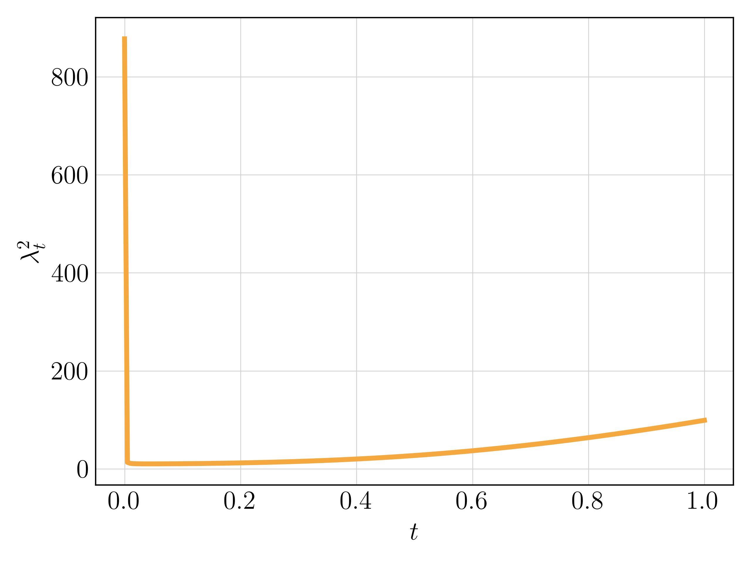
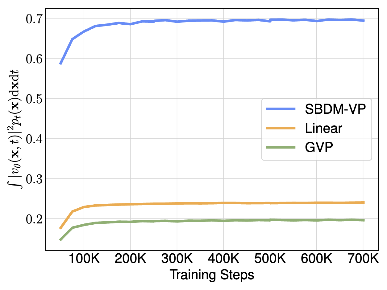
As \(t \to 0\), \(\dot \sigma_t \to -\infty\) under the variance preserving setting, making \(\lambda_t^2\) blow up to infinity as well. In practice, we follow the setting of SBDM and clip both training and sampling to the interval \([\varepsilon, 1]\) to avoid numerical stability.
As a result, the large \(\lambda_\varepsilon\) is able to compensate for the vanishing gradient of \(\mathcal{L}_s\), but in turn makes \(\mathcal{L}_v\) harder to optimize.
We mainly experiment with three choices of interpolants:
| Interpolant | Objective | FID |
|---|---|---|
| SBDM-VP | \( \mathcal{L}_v\) | 39.8 |
| GVP | \( \mathcal{L}_v \) | 34.6 |
| Linear | \( \mathcal{L}_v \) | 34.8 |
We introduce more flexibility in sampling the velocity model in this section. Firstly, under SBDM setting, the reverse-time SDE for velocity can be constructed in the following way: \[
dX_t = [v(X_t, t) - \frac12 g^2(t)s(X_t, t)]\mathrm{d}t + g(t) \mathrm{d} \bar{W}_t
\]
where we take advantage of the linear relationship between velocity and score to construct the drift term. We denote \(g(t)\) as the SBDM diffusion coefficient.
Following previous sections, we can also construct such SDE for GVP and Linear interpolants given the relationship \(g^2(t) = 2\lambda_t\sigma_t\). The results are resented below
Interpolant
Objective
ODE
SDE
SBDM-VP
\( \mathcal{L}_v\)
39.8
37.8
GVP
\( \mathcal{L}_v \)
34.6
32.9
Linear
\( \mathcal{L}_v \)
34.8
33.6
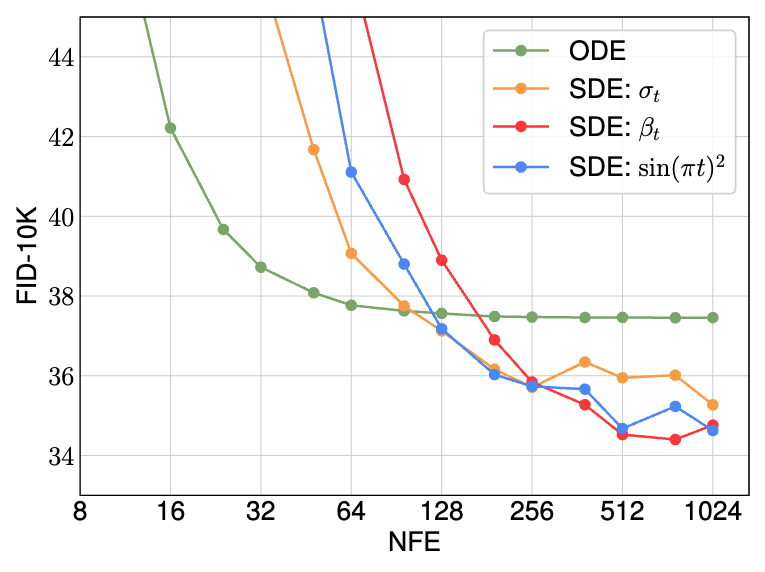
We further proposed that the diffusion coefficient \(g(t)\) can be tuned separately from the learning process. In fact, any non-negative function \(w(t)\) (not necessarily monotone) is eligible to be used as diffusion coefficient, and the reverse-time SDE can thus be generalized to \[
dX_t = [v(X_t, t) - \frac12 w(t)s(X_t, t)]\mathrm{d}t + \sqrt{w(t)} \mathrm{d} \bar{W}_t
\]
Apart from SBDM coefficient, we also experiment with the choices of \(w(t) = \sigma_t\) (to eliminate the singularity of score near data distribution) and \(w(t) = \sin^2(\pi t)\), as well as their effects on either velocity or score models.
Interpolant
Objective
\( w(t) = g(t)\)
\( w(t) = \sigma_t \)
\( w(t) = \sin^2(\pi t)\)
SBDM-VP
\( \mathcal{L}_v\)
37.8
38.7
39.2
\( \mathcal{L}_{s_\lambda}\)
35.7
37.1
37.7
GVP
\( \mathcal{L}_v \)
32.9
33.4
33.6
\( \mathcal{L}_s \)
38.0
33.5
33.2
Linear
\( \mathcal{L}_v \)
33.6
33.5
33.3
\( \mathcal{L}_s \)
41.0
35.3
34.4
We note that the optimal choice of diffusion coefficient depends on the interpolant and the objective, and in our experiments, also largely depends on model sizes. Empirically, we observe the best choice for our SiT-XL is a continuous-time velocity model with Linear interpolant and sampled using SDE with \(w(t) = \sigma_t\) coefficient.
Lastly, we note that the performance of ODE and SDE integrators may differ under different computation budget. As shown below, the ODE converges faster with fewer number of functions evaluations, while the SDE is capable of reaching a much lower final FID score when given a larger computational budget.
In this section, we give a concise justification for adopting it on the velocity model, and then empirically show that the drastic gains in performance for DiT case carry across to SiT.
Guidance for a velocity field means that: (i) that the velocity model \(v_\theta(x_t, t, y)\) takes class labels \(y\) during training, where \(y\) is occasionally masked with a null token \(\emptyset\); and (ii) during sampling the velocity used is \(v_\theta^\zeta(x_t, t, y) = \zeta v_\theta(x_t, t, y) + (1 - \zeta) v_\theta(x_t, t, \emptyset)\) for a fixed \(\zeta > 0\). Given this observation, one can leverage the usual argument for classifier-free guidance on score-based models. For a CFG scale of \(\zeta = 1.5\), DiT-XL sees an improvement in FID from a 9.6 (non-CFG) down to 2.27 (CFG). We observed similar performance improvement with our largest SiT-XL model under identical computation budget and CFG scale. Sampled with an ODE, the FID-50K score improved from 9.4 to 2.15; with an SDE, the FID improved from 8.6 to 2.06. This shows that SiT benefits from the same training and sampling choices explored previously, and can surpass DiT's performance in each training setting, not only with respect to model size, but also with respect to sampling choices.
| Class-Conditional ImageNet \(256\times256\) | |||||
|---|---|---|---|---|---|
| Model | FID \(\downarrow\) | sFID \(\downarrow\) | IS \(\uparrow\) | Precision \(\uparrow\) | Recall \(\uparrow\) |
| BigGAN-deep |
6.95 | 7.36 | 171.4 | 0.87 | 0.28 |
| StyleGAN-XL |
2.30 | 4.02 | 265.12 | 0.78 | 0.53 |
| Mask-GIT |
6.18 | - | 182.1 | - | - |
| ADM |
10.94 | 6.02 | 100.98 | 0.69 | 0.63 |
| ADM-G, ADM-U | 3.94 | 6.14 | 215.84 | 0.83 | 0.53 |
| CDM |
4.88 | - | 158.71 | - | - |
| RIN |
3.42 | - | 182.0 | - | - |
| Simple Diffusion(U-Net) |
3.76 | - | 171.6 | - | - |
| Simple Diffusion(U-ViT, L) | 2.77 | - | 211.8 | - | - |
| VDM++ |
2.12 | - | 267.7 | - | - |
| DiT-XL(cfg=1.5) | 2.27 | 4.60 | 278.24 | 0.83 | 0.57 |
| SiT-XL(cfg=1.5, ODE) | 2.15 | 4.60 | 258.09 | 0.81 | 0.60 |
| SiT-XL(cfg=1.5, SDE:\(\sigma_t\)) | 2.06 | 4.50 | 270.27 | 0.82 | 0.59 |
In this work, we have presented Scalable Interpolant Transformers, a simple and powerful framework for image generation tasks. Within the framework, we explored the tradeoffs between a number of key design choices: the choice of a continuous or discrete-time model, the choice of interpolant, the choice of model predcition, and the choice of samplers . We highlighted the advantages and disadvantages of each choice and demonstrated how careful decisions can lead to significant performance improvements. Many concurrent works
@article{ma2024sit,
title={SiT: Exploring Flow and Diffusion-based Generative Models with Scalable Interpolant Transformers},
author={Nanye Ma and Mark Goldstein and Michael S. Albergo and Nicholas M. Boffi and Eric Vanden-Eijnden and Saining Xie},
year={2024},
eprint={2401.08740},
archivePrefix={arXiv},
primaryClass={cs.CV}
}